Hello, World!

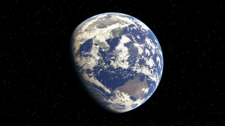
When learning a new language, it’s traditional for programmers to write a first program that simply prints out, “Hello, World!”. Since I am a programmer writing my first blog entry on a real-time rendering topic, I decided to say “hello” by ‘rendering the world’.

Recently, I’ve been researching atmospheric scattering for use in large, outdoor virtual environments such as games, simulations, or virtual reality experiences. To continue exploring the subject, I wanted to choose a few experiences to test them in, implement some of the published rendering techniques, and evaluate the results to see what works best.

I’ve chosen three experiences that I believe should lend well to either the screen or virtual reality:

• Space cockpit simulation
• Atmospheric flight simulation
• Driving/racing simulation.

Since this blog entry is about rendering the world from space, I’ll only be discussing an atmospheric scattering technique useful for the space cockpit simulation, e.g. planets, moons, celestial objects, etc., as seen from space.

For my simulation, I made up some requirements for rendering Earth:

• The simulation shall be capable  of rendering the Earth from variable orbit (say between low Earth Orbit (LEO) and the moon)
• The simulation shall be capable of modeling time-of-day (day/night)
• The simulation shall be capable of modeling time-of-year (seasons)
• The simulation shall render a ‘reasonable’ approximation of atmospheric scattering

The first three requirements are easily solvable, that is, for a low-fidelity, non-mission critical, entertainment experience. I will, therefore, keep it simple by assuming perfectly circular orbits and spheres for all planetary bodies.

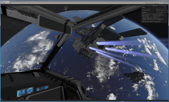
The problem will still be an exercise in fitting the scale of the inner solar system into reference frames that fit within the computer’s floating point accuracy. If you’ve ever tried, you’ve likely encountered the ‘jitter’, stemming from insufficient floating-point precision that exists when rendering the solar system to scale in a single reference frame [Cozzi and Ring 11]. In order to combat jitter, I will be using a multiple layer camera system in my cockpit simulation to render each reference frame, which includes one for each of the following:

• Cockpit interior
• Local Frame: ‘Combat-zone’ or ‘Battle-space’
• Planet Frame: (Earth)
• Universe Frame: Moon/sun/stars, and other solar system planets

The rendering order is bottom-to-top, in this case, with the first-person, cockpit interior being rendered last against the depth buffer.

The rest of this blog entry is about solving the last requirement, that is, rendering a ‘reasonable’ approximation of atmospheric scattering (Earth from Space).

In researching various atmospheric scattering techniques, both online as well as published articles in text books, I’ve come across two real-time techniques that I wanted to try out. The first was developed by [O’Neil 05]. This technique can be tailored to suit atmospheric scattering from ‘space-to-ground’ or ‘ground-to-space’. I have had great results using this technique, for both my driving simulation as well as space-cockpit simulations. I hope to show both of those off in a later blog post.

The other technique I found is [Schüler 12]. The paper describes a real-time algorithm to render the ‘aerial perspective’ phenomenon, and it details the approximations methods taken to perform this algorithm in real-time. I wanted to share some my results from implementing a custom Cg/HLSL planet shader to render the Earth from space, with the aerial-perspective based on Schüler’s technique.

 

Night to Day Video

Day to Night Video

User Interface Video

I’m using Unity as my shader sandbox, making sure to turn off all default lighting, shadows, post-processing, etc. within the Unity Editor to ensure that the only colors being rendered to the screen are from my shaders.

Vertex Shader

For this algorithm, all of the lighting calculations are performed in model (or object) space. Unity provides us with a world light position and world camera position (_WorldSpaceLightPos0 and _WorldSpaceCameraPos respectively), which I transform to model space using the unity matrix helper function, unity_WorldToObject. Doing this allows me to move the light and camera programmatically at run-time using the Unity editor, in-game user interface, or game controller script.

Below is the entire vertex shader:

v2f vert (appdata v)
{
   v2f o;
   o.vertexPos = v.vertex;
   o.cameraPos = mul(unity_WorldToObject, float4(_WorldSpaceCameraPos.xyz, 1));
   o.lightDir = mul(unity_WorldToObject, _WorldSpaceLightPos0).xyz;
   o.vertex = UnityObjectToClipPos(v.vertex);

   // compute bitangent from cross product of normal and tangent
   half3 bitangent = cross(v.normal, v.tangent) * v.tangent.w;

   // output the tangent space matrix
   o.tspace0 = half3(v.tangent.x, bitangent.x, v.normal.x);
   o.tspace1 = half3(v.tangent.y, bitangent.y, v.normal.y);
   o.tspace2 = half3(v.tangent.z, bitangent.z, v.normal.z);

   return o;
}

The vertex position is already in model space, so it simply gets passed to the fragment shader. The vertex shader also transforms the vertex to clip space as required by a vertex shader. Additionally, in order to use the normal map for the planet surface, I output the normal, tangent, and bitangent in model space as well.

Here are my vertex shader inputs and semantics:

struct appdata
{
   float4 vertex : POSITION;
   float3 normal : NORMAL;
   float4 tangent : TANGENT;
};

Here are my vertex shader outputs and semantics:

struct v2f
{
   float4 vertex : SV_POSITION;
   float4 vertexPos : TEXCOORD0;
   float4 cameraPos : TEXCOORD1;
   float3 lightDir : TEXCOORD2;

   half3 tspace0 : TEXCOORD3; // tangent.x, bitangent.x, normal.x
   half3 tspace1 : TEXCOORD4; // tangent.y, bitangent.y, normal.y
   half3 tspace2 : TEXCOORD5; // tangent.z, bitangent.z, normal.z
};

Fragment Shader

The first step of the fragment shader is to perform a raycast against the implicit sphere of the planet. By implicit, I mean the equation of a sphere of a given radius, not the  radius of the actual geometry of the sphere model. For example, the sphere model may be a radius of 1.0, but the radius of the implicit sphere might be something like 0.9, giving up 10% to rendering the exponentially decaying atmosphere. I typically am using something more like 0.94 for the implicit radius and passing that value in from my application.

fixed3 col = fixed3(0,0,0);
float alpha = 1.0;

// .. local variables ..
float4 P = pointOnSphereSurface(camPos, viewDir, _radius);
if (P.w == 0.0)
{
   // no surface intersection.
   float3 T, S;
   aerialPerspective(T, S, camPos, camPos + viewDir, true, lightDir);
   col = S;

   // Doing alpha blending in the atmosphere.
   alpha = 0.0;
}
else
{
   // .. perform algorithm against planet ray-intersect
}

The fragment shader calls the function pointOnSphereSurface from the camera position in along the view direction (both in model space), and it returns the point on the implicit sphere that it intersected. If no intersection occurs, the algorithm then calls the aerialPerspective function against the infinite backdrop of space to calculate the color of any atmosphere present. I also set the alpha of the color to zero, so that I can alpha blend the stars and/or sun behind the atmosphere (otherwise you would see a thick black circle around the planet, which is only fine if you aren’t rendering a background).

For the pointOnSphereSurface function, I used a math textbook and implemented the intersection of a ray and a sphere. One such source is [Lengyel 12]. The ‘a’ term drops out in the discriminant calculation in the code below because we are using a normalized view direction [Sellers 14], so a = dot(V, V) = 1.0, because the length of the view vector is one. Here is my code for that method:

float4 pointOnSphereSurface(float3 S, float3 V, float radius)
{
   // Interset a point on an implicit surface.
   float4 result = float4(0, 0, 0, 0);

   float r = radius;
   float R2 = r * r;
   float S2 = dot(S, S);

   // a = dot(V, V) = 1.0, because V the normalized view direction.
   float b = 2.0 * dot(S, V);
   float c = S2 - R2;

   // Discriminant = b^2 - 4ac
   // We only need: b^2 - 4c, a = 1.0
   float D = b * b - 4.0 * c;

   if (D >= 0.0)
   {
      if (S2 > R2) // camera outside the surface
      {
         float t = (-b - sqrt(D)) * 0.5;

         if (t > 0.0)
         {
            result = float4(S + V * t, 1);
         }
      }
      else // camera on the surface
      {
         result = float4(S, 1);
      }
   }
   return result;
}

Note that the key to this is that the Discriminant (D) tells you if an intersection occurs, and only if it is greater or equal to zero do we need to bother with taking a square root. We are raytracing in real time in our pixel shader, so we want to avoid such calculations unnecessarily.

Please see [Schüler 12] for the aerial perspective shader code function, as it is available from the book’s website as a download. The function returns two colors, T and S, where T represents the amount of light transmitted back to the viewer and S represents the light due from scattering. I only use one light, so the final color can be represented by:

C = S + ( T ) * ( surface color)

I also refer you to [Schüler 12] for the transmittance function, which yields the light color, that is the color of light to the observer through the atmosphere. It uses Schüler’s efficient approximation to the Chapman function, explained in his publication. The lightColor will be used to affect the planet’s surface color, ocean color, and cloud color.

   float3 lightcolor = transmittance(P.xyz, lightDir);

Now to the case where our raycast intersects with, or is on, the implicit sphere. The first step is to normalize the point returned and generate spherical UV coordinates so that we can sample the textures. My textures all map to the same sphere model, so I only need one set of UVs. Note that this UV texture mapping is for DirectX rendering and not OpenGL.

   float3 N = normalize(P.xyz);
   float2 uv = float2(0.5, 0.5) + float2(.15915494, .31830989) * float2(atan2(N.z, N.x), asin(N.y));

   // sample the surface texture and
   float3 surfacecolor = tex2D(_EarthColor, uv).xyz;

Next, I sample the normal map using Unity’s UnpackNormal helper.

// sample the normal map, and decode from the Unity encoding
half3 mapNormal = UnpackNormal(tex2D(_BumpMap, uv));

// transform normal from tangent to object space
half3 landNormal;
landNormal.x = dot(i.tspace0, mapNormal);
landNormal.y = dot(i.tspace1, mapNormal);
landNormal.z = dot(i.tspace2, mapNormal);

We can shade the land using the Lommel-Seeliger Law. Note that NdotL and NdotV are using the normal map instead of the normal from the implicit sphere intersection. The land is the only item I want to do bump mapping on, so I recalculate NdotL and NdotV afterwards, using the implicit normal, to use for the rest of the algorithm.

// for shading the landmass we use the Lommel-Seeliger law
float3 V = -viewDir;
float dotNV = max(0.0, dot(landNormal, V));
float dotNL = max(0.0, dot(landNormal, lightDir)); // Note: using normal map here.
float3 landcolor = 1.5 * lightcolor * surfacecolor * dotNL / (dotNL + dotNV);

// Note: recaclulate NdotL and NdotV using sphere normal for the rest of the calcs.
dotNL = max(0.0, dot(N, lightDir));
dotNV = max(0.0, dot(N, V));

Next, I shade the ocean as described by [Schüler 12] , which incorporates the surface map, calculated sky color (using the reflection vector), and a fresnel factor. Specular reflection on the ocean is rendered using the technique in [Schüler 09].

I calculate a cheap cloud color to add in to the lighting model from a texture map. I arrived at this by experimentation, and I consider it a work-in-progress.

// Factor in the clouds. This is mostly experimentation to get my cloud texture to look convincing.
float3 cloudColor = 3.0 * tex2D(_Clouds, uv);
float3 finalCloudColor = 1.5 * cloudColor * lightcolor * dotNL / (dotNL + dotNV);

The final for the lighting model is to call aerialPerspective function from the camera’s point of view and then obtain the final color. This will be the S, scattered light, added to the transmittance factor multiplied with the surface and cloud color.

aerialPerspective(T, S, camPos, P.xyz, false, lightDir);

// Final color model
col = S + T * (surfacecolor + finalCloudColor);

I take a similar approach as [Schüler 12] does in performing a final tone mapping and saturation control to the output color.

Unfortunately, in terms of gamma correction, I’m not certain of the state of the input textures and exactly how the Unity Engine handles this. I am Unity’s Linear path, and I’ve set my input textures to Linear, as opposed to sRGB. I am also using alpha blending. My final two statements are:

col = pow(col, 2.2);
return fixed4(col.xyz, alpha);

I found that this gave me results I liked, but may not be correct in terms of how gamma correction is done, however my color output was simply too bright and faded without the 2.2 power function.

For the alpha blend function, I’m using:

Blend One OneMinusSrcAlpha

This allows me to add backgrounds behind the Earth, such as a procedural GPU rendered star field, skybox, sun, moon, etc, without seeing a black outline around the planet model where the atmosphere is zero. My sun and stars are using additive blending. I’ve found that it looks more realistic with no star field, as the intensity of the lit planet would make the stars invisible. But for animation purposes, or dramatic effect, I want the option to alpha blend these into my scene.

There’s plenty more work to be done to complete my cockpit simulation. I can now render in real-time, an Earth that satisfies all of my requirements, including dynamic and configurable atmospheric scattering. I will review my implementation of [O’Neil 05] and see how it looks and performs in comparison to [Schüler 12]. I am eager to see how they both look in virtual reality as well as in my multi-camera system that includes a cockpit and a few other ships in my ‘battle-space’ layer.

Besides correcting any mistakes, for improvement, I also would like to:

• Use higher resolution textures
• Add city lights to night
• Render clouds above the planet, and with shadows
• Add a sun flare effect
• Add post processing effects
• Implement a level-of-detail
• Add the moon and a lighting model that utilizes it
• Implement a star field that changes intensity wrt time-of-day (planet lit or dark)

So, that’s it for my first blog post, and I learned a lot to get this far. I suspect I will learn quite a bit more to improve my blogging skills.

Thanks for reading, and Hello, World!

Bibliography

[Cozzi and Ring 11] Patrick Cozzi and Kevin Ring. “Vertex Transform Precision.”  In 3D Engine Design for Virtual Globes, Chapter 5, pp 157-180. Boca Raton, FL: CRC Press, 2011.

[Lengyel 12] Eric Lengyel.  “Ray Tracing.” In Mathematics for 3D Game Programming and Computer Graphics Third Edition, Chapter 6.2.3, pp. 144-145. Boston, MA: Course Technology, a part of Cengage Learning, 2012.

[O’Neil 05] Sean O’Neil.  “Accurate Atmospheric Scattering.” In GPU Gems 2, edited by Matt Pharr and Randima Fernando, pp. 253-268. Reading, MA: Addison-Wesley, 2005.

[Schüler 12] Christian Schüler. “An Approximation to the Chapman Grazing-Incidence Function for Atmospheric Scattering.”  In GPU Pro 3 : Advanced Rendering Techniques, edited by Wolfgang Engel. Chapter 2.2, pp. 105-118. Boca Raton, FL: CRC Press, 2012.

[Schüler 09] Christian Schüler. “An Efficient and Physically Plausible Real-Time Shading Model.”  In ShaderX 7 : Advanced Rendering Techniques, edited by Wolfgang Engel, Chapter 2.5, pp. 175-187. Hingham, MA: Charles River Media, 2009.

[Sellers, Wright, and Haemel 14] Graham Sellers, Richard S. Wright, Jr., and Nicholas Haemel.  “Rendering Techniques.”  In OpenGL SuperBible Sixth Edition, Chapter 12, pp 569-580. Upper Saddle River, NJ: Addison-Wesley, 2014.